Unsteady Vortex Lattice Method (UVLM)

We model the aerodynamics using the unsteady vortex lattice method (UVLM), which allows for time domain aerodynamic predictions under the assumption of low speed attached flows and enables arbitrary deformations. The UVLM allows for lifting aerodynamic bodies to be represented as panels with no thickness. A summany of the numerics is presented here, however, are given in more detail by Katz and Plotkin.

We here use subscript \(\bullet_b\) to denote a bound grid quantity, and \(\bullet_w\) to denote a wake property. For a given strip on the aerodynamic grid, we can obtain the inertial coordinates and velocities of its \(i\)-th node as a function of the structural coordinates and time derivatives

\[ \begin{Bmatrix} \pmb{\zeta}_{b, ij} \\ 1 \end{Bmatrix} = \mathbf{H}_j \begin{Bmatrix} \pmb{\zeta}_{b0, ij} \\ 1 \end{Bmatrix} \]

\[ \begin{Bmatrix} \dot{\pmb{\zeta}}_{b, ij} \\ 1 \end{Bmatrix} = \dot{\mathbf{H}}_j \begin{Bmatrix} \pmb{\zeta}_{b0, ij} \\ 1 \end{Bmatrix} \]

where \(\mathbf{H}_j\) is the \(j\)-th beam node SE (3) coordinate, and \(\pmb{\zeta}_{b0}\) gives the aerodynamic grid coordinates in the local frame of reference, with a representation of an aerodynamic bound and wake grid shown below. This grid is set when setting the design variables of a UVLM instance with the zeta_b0 input.

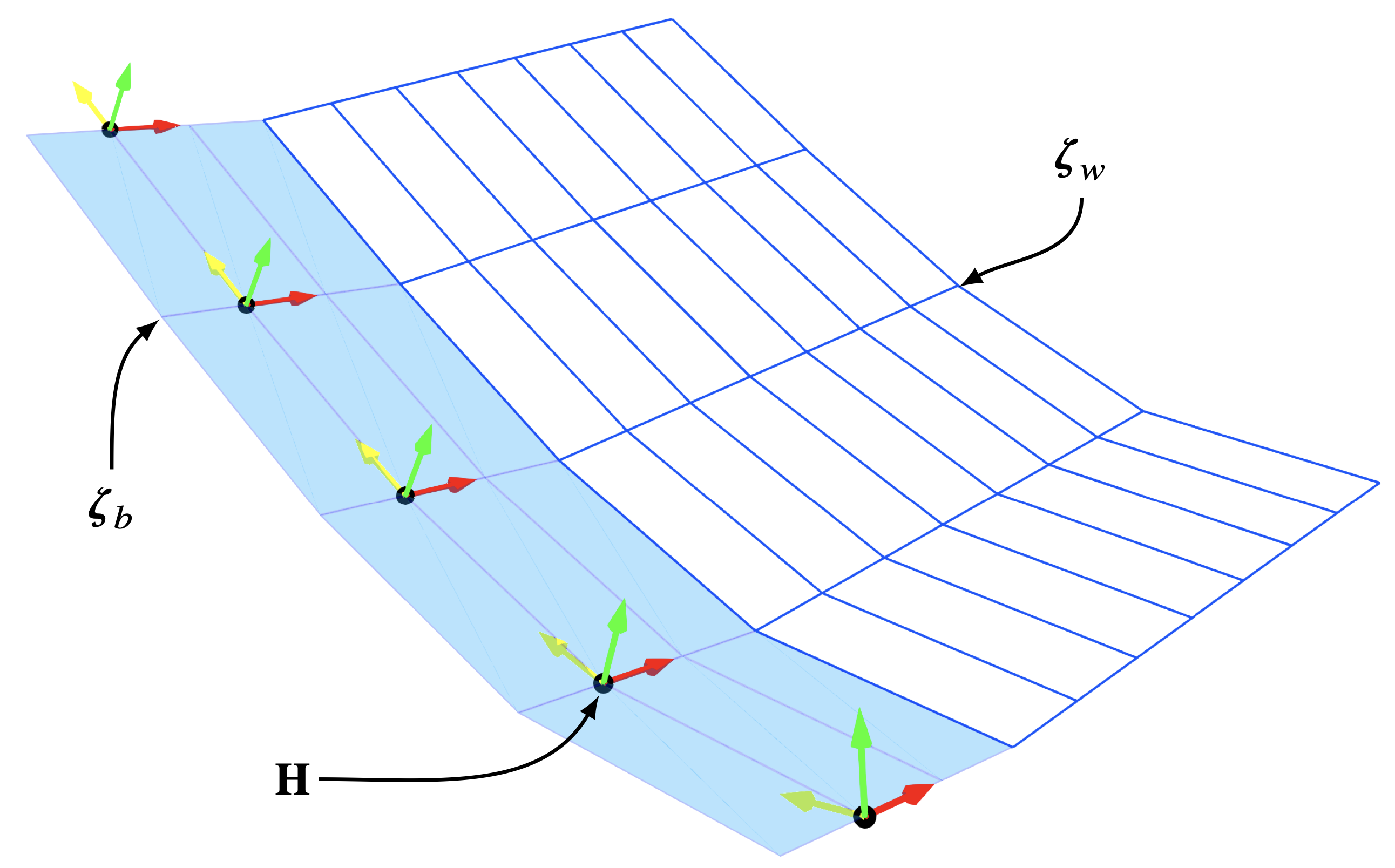Representative aerodynamic geometry for the UVLM mapped onto a deformed beam. The local grid coordinates $$

For the steady vortex lattice method (VLM) problem, the aerodynamic system can be solved by enforcing flow tangential to the body at collocation points \(\pmb{\zeta}_c\), which are chosen to be at the centre of the aerodynamic panels

\[ \left (\pmb{\mathcal{A}} \pmb{\Gamma}_b + \pmb{\nu}_{\infty}\right) \cdot \mathbf{n} = \mathbf{0} \]

where \(\pmb{\mathcal{A}}\) is the aerodynamic influence matrix (AIC), which maps the influence of each vortex ring to each collocation point; \(\mathbf{\Gamma}_b\) is a vector of bound panel circulation strengths, and \(\pmb{\nu}_{\infty}\) is the velocity induced by the freestream at the collocation points. This solution is projected onto the surface normals \(\mathbf{n}\), which are obtained as a function of the bound grid coordinates \(\pmb{\zeta}_b\). As circulation is propagated from the training edge of the bound body into the wake to satisfy the Kutta condition, this infers a constant circulation strength along wake streamlines for a steady case. As such, the wake influence can be summed into the trailing edge influence in matrix \(\pmb{\mathcal{A}}\). This system can be readily solved for \(\mathbf{\Gamma}_b\).

From this solution, steady aerodynamic forcing can be obtained for each filament vector \(\mathbf{k}_0^{\text{filament}}\) on the grid

\[ \mathfrak{f}^{\text{filament}}_{\text{steady}} = \rho \Gamma \pmb{\nu} \times \mathbf{k}_0^{\text{filament}} \]

where velocity \(\pmb{\nu}\) is evaluated at the midpoint of the given filament, and it includes contributions from both the freestream and the vortex filaments. The circulation \(\Gamma\) here refers to the effective circulation; for filaments shared between two vortex rings, this is the difference in the circulation strengths of the rings. The forcing can be split from filament midpoints to being at the aerodynamic grid nodes before being projected onto the beam and transformed into the local frame of reference to obtain forces and moments for compatibility with the structural equations as

\[ \mathbf{f}_{\text{aero}, j} = \sum_{i=1}^{m} \begin{Bmatrix} \mathbf{R}^{\top}_j \, \mathfrak{f}_{\text{steady}, ij} \\ \pmb{\zeta}_{0, ij} \times \left (\mathbf{R}^{\top}_j \, \mathfrak{f}_{\text{steady}, ij}\right) \end{Bmatrix} \]

with \(\mathfrak{f}\) used to denote aerodynamic forcing on the aerodynamic grid, and \(\mathbf{f}\) being projected onto the beam.

For the unsteady case, we introduce lag terms from the wake that need to be captured, as the current UVLM solution depends on data from the previous step. The aerodynamic system can be solved as

\[ \left (\pmb{\mathcal{A}}_b \pmb{\Gamma}_b + \pmb{\mathcal{A}}_w \pmb{\Gamma}_w + \pmb{\nu}_{\infty} - \dot{\pmb{\zeta}}_c\right) \cdot \mathbf{n} = \mathbf{0} \]

where \(\pmb{\mathcal{A}}_b\) and \(\pmb{\mathcal{A}}_w\) are AIC matrices mapping from the bound and wake aerodynamic grids to the collocation points, respectively, as these are not combined as in the steady case. Here \(\dot{\pmb{\zeta}}_c\) is the velocity of the collocation points, found from the interpolation of \(\dot{\pmb{\zeta}}_b\). Computing the steady forcing requires including the velocity of the bound grid to find the velocity of the flow relative to the filament midpoint, but it is otherwise unchanged. As we consider apparent mass effects, unsteady forcing for a single panel is given as

\[ \mathfrak{f}_{\text{unsteady}}^{\text{panel}} = \rho \dot{\Gamma} S \mathbf{n} \]

where the forcing can be split from the panel centroid to its surrounding grid nodes and projected onto the beam, as with the steady forcing. The time derivative of circulation can lead to instabilities when coupled with a dynamic structure due to a feedback loop created between structural acceleration and unsteady aerodynamic forcing. To remedy this, we filter the derivative as

\[ \dot{\mathbf{\Gamma}}_{n} \approx \frac{g}{h} \left (\mathbf{\Gamma}_n - \mathbf{\Gamma}_{n-1}\right) + (1-g) \dot{\mathbf{\Gamma}}_{n-1} \]

where the choice to use first-order differences is made for convenience in the resulting tangent problem by only referring to one previous timestep, with \(g\) as a filtering parameter. When using the code this parameter is set through gamma_dot_relaxation when creating a UVLM instance, with a default value of 0.7.

The UVLM requires that circulation be convected into the wake, which introduces memory into the system. Two options for the convection scheme have been implemented:

\[ \mathbf{\Gamma}_{w, n} = \pmb{\mathcal{W}}_{\Gamma} (\mathbf{\Gamma}_{b, n-1}, \mathbf{\Gamma}_{w, n-1}) \]

\[ \pmb{\zeta}_{w, n} = \pmb{\mathcal{W}}_{\zeta} (\pmb{\zeta}_{b, n}, \pmb{\zeta}_{w, n-1}) \]

Firstly there is the base scheme, which shifts both the wake grid and circulation strengths downstream by one panel length per timestep, resulting in a Courant–Friedrichs–Lewy number of one. This results in all wake panels having approximately the same length along the streamwise direction. Whilst this method is simple, it requires a large number of panels to construct a long wake, which can prove expensive. Alternatively, a variable-discretisation can be used. This allows for wake streamlines to have an arbitrary discretisation, where both the coordinates and circulation strengths are shifted downstream before being projected back onto a given discretisation. This allows for larger panels far downstream in the wake, which has shown a reduction in computational costs with minimal loss in accuracy. These can be toggled by settting variable_wake_disc when creating a UVLM instance. When using a variable discretisation, we must set delta_w when setting the design variables; this is a vector which encodes the length of each wake segment, from upstream to downstream.

For both wakes types, there are two methods for convecting the wake coordinates \(\pmb{\zeta}_w\). By default we use a prescribed wake convected between time steps using only the background velocity. Alternatively, a free wake can be used, which also includes induced velocity from the vortex and results in a characteristic roll-up. However, a free wake adds considerable computational cost for only a small change in the results and is often omitted. These can be toggled by setting the free_wake parameter when creating a UVLM instance.

Compressibility correction (Prandtl-Glauert)

The UVLM is otherwise incompressible. A subsonic compressibility correction can be applied by setting mach on a FlowField instance (default 0, i.e. incompressible), which defines the Prandtl-Glauert factor \(\beta = \sqrt{1 - M^2}\). The correction uses the rigorous 3D Prandtl-Glauert-Göthert transform: components of the aerodynamic grid parallel to the freestream direction are left unchanged, while components perpendicular to the freestream are scaled by \(\beta\),

\[ \pmb{\bar{\zeta}} = \pmb{\zeta}_\parallel + \beta \pmb{\zeta}_\perp \]

The AIC matrix, boundary condition, and bound/wake circulation solve are all performed on this transformed geometry, exactly as for the incompressible problem, giving a transformed circulation \(\bar{\mathbf{\Gamma}}\). The physical circulation is then recovered via Göthert's rule

\[ \mathbf{\Gamma} = \bar{\mathbf{\Gamma}} / \beta^2 \]